How to Design a Metrics Collector System

1. Functional Requirements

Multi-source Collection: Ingest metrics from diverse sources, including application servers, databases, and middlewares.
Flexible Ingestion Models: Support both Push and Pull models for data collection.
Data Transformation: Capabilities for parsing, filtering, and enriching metrics with labels (tags/metadata).
Persistent Storage: Scalable storage for time-series data with high-resolution timestamps.
Query API: Provide a robust API to power frontend dashboards (e.g., Grafana).
Alerting & Notification: Evaluate predefined threshold rules and trigger alerts through various channels (Slack, Email, PagerDuty).

Write-Heavy Architecture: Optimize for high-throughput data ingestion.
Scalability: Horizontal scalability for both the ingestion layer and the storage engine.
High Availability: Ensure the system remains operational despite component failures.
Storage Efficiency: Use advanced compression and downsampling to manage long-term data growth.
Reliability: Guarantee eventual consistency, which is generally sufficient for monitoring use cases.

Total Metrics: $10,000,000$ unique metrics.
Data Points Per Second (DPS): $10,000,000 / 10 \text{ s} = 1,000,000 \text{ DPS}$.
QPS (Batching): Assuming a batch size of 100 metrics per request, the effective ingestion QPS is $1,000,000 / 100 = 10,000 \text{ QPS}$.

Bandwidth: $1,000,000 \text{ DPS} \times 50 \text{ B} = 50 \text{ MB/s}$ (approx. $400 \text{ Mbps}$).
Raw Storage (Daily): $50 \text{ MB/s} \times 86,400 \text{ s} \approx 4.32 \text{ TB/day}$.
Raw Storage (Annual): $4.32 \text{ TB} \times 365 \approx 1.57 \text{ PB/year}$.
With Optimization: By applying TSDB compression (e.g., Gorilla XOR/Delta-of-Delta, ~90% reduction) and Downsampling, the annual storage footprint can be reduced to a manageable ~50 TB.

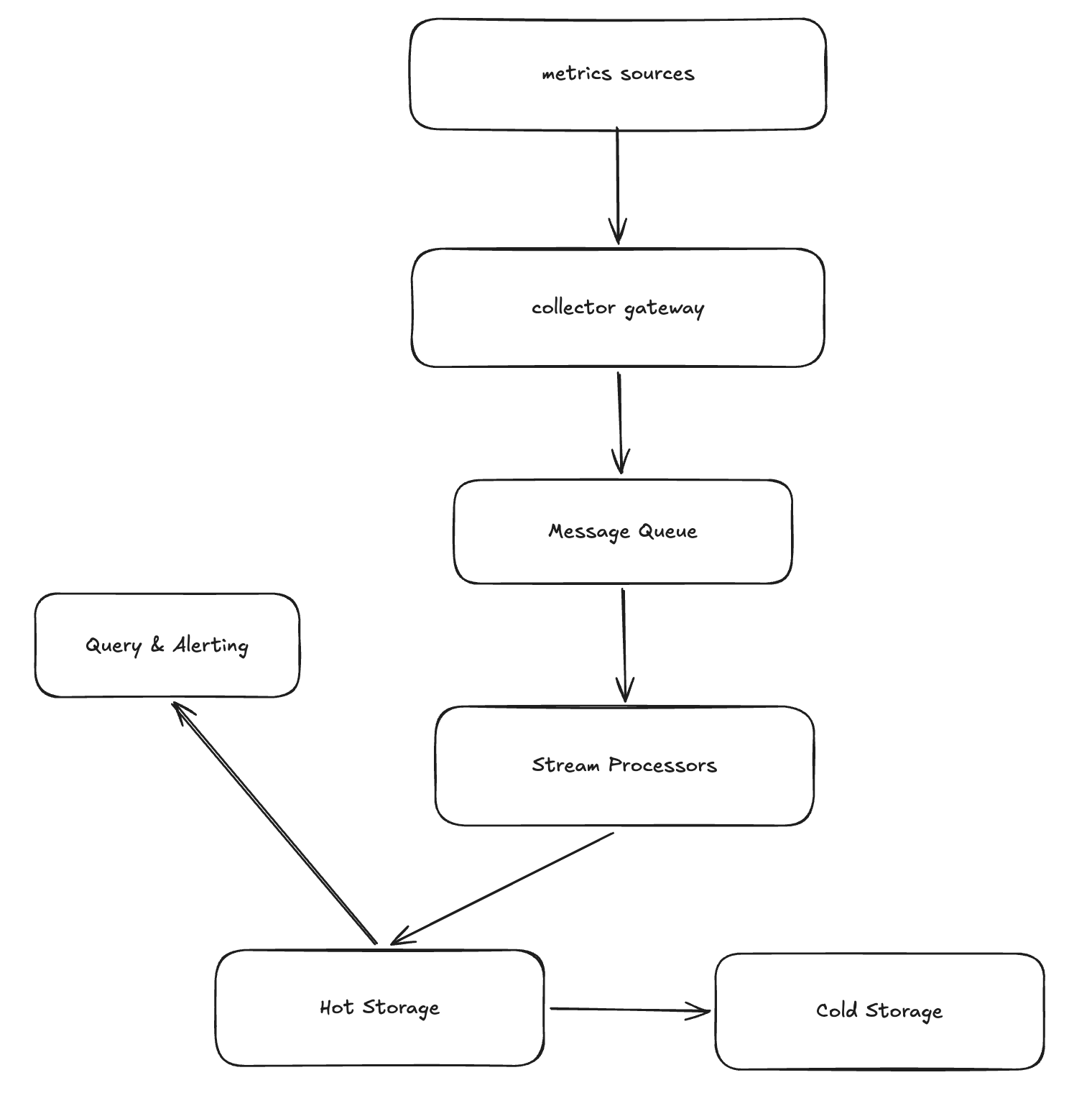
High Level Design

How do we handle potential traffic spikes and ensure system stability?

Pull Model (e.g., Prometheus): The collector proactively scrapes metrics. This provides inherent back-pressure as the collector controls the scraping rate, preventing the system from being overwhelmed. However, it requires a service discovery mechanism to track all targets.
Push Model (e.g., StatsD): Agents send data to a gateway. This is easier to scale and works well for short-lived jobs (serverless), but the gateway can be vulnerable to “thundering herd” floods without a robust load balancer and message queue.

Why use a Time Series Database (TSDB) instead of a traditional RDBMS like MySQL?

LSM-Tree vs. B+ Tree: Metrics are write-heavy. LSM-Trees (used in InfluxDB/Prometheus) convert random writes into sequential disk I/O, offering significantly higher write throughput than the B+ Trees used in traditional relational databases.
Gorilla Compression (Facebook):
- Timestamp Compression (Delta-of-Delta): Since collection intervals are usually fixed (e.g., every 10s), the “difference of differences” is often zero, which can be stored in just 1 bit.
- Value Compression (XOR): Floating-point values typically change very little between consecutive samples. XORing consecutive values allows us to store only the significant bits, drastically reducing the storage footprint.

To balance query performance and storage costs, we aggregate older data.

Stream Processing: Aggregates data in real-time as it is ingested (e.g., via Flink). This offers low latency for alerts but increases architectural complexity (handling late-arriving data via watermarks).
Batch Processing: Aggregates data periodically (e.g., hourly/daily) using Spark or MapReduce. While simpler to implement, it creates a “lag window” for aggregated queries and can cause heavy read pressure on the hot storage layer during the batch run.